I spent last weekend fine-tuning an embedding model on a single RTX 3090, which is a sentence I would have laughed at in 2024, when the accepted wisdom was that retrieval quality came from renting the biggest embedding API you could afford. Then Sentence Transformers v6.0 shipped MultiVectorEncoder, Tom Aarsen published a training guide for it on the Hugging Face blog, and the numbers in it rearranged some of my assumptions about how retrieval stacks should be built. A 0.3B model, fine-tuned overnight on consumer hardware, beating an embedding model with roughly 33x the active parameters. On the right benchmark, sure. But still.
Short version for the impatient: late-interaction models are now first-class citizens in the most boring, well-supported embedding library there is, fine-tuning one on your own domain is cheap, and the punishing index sizes that made everyone ignore ColBERT for years have workable fixes. The longer version has numbers.
What multi-vector actually means
A regular dense embedding model reads your text and compresses everything into one vector. One vector per document, one dot product per comparison, tidy and fast. The price is that the compression is lossy in exactly the way that hurts retrieval: rare terms, specific numbers, and fine distinctions get averaged into mush.
A multi-vector model (ColBERT-style, also called late interaction) keeps one small vector per token instead. At query time, each query token searches the document’s tokens for its best match, and those best-match scores get summed. The operation is called MaxSim, and the practical effect is that a query about “grade 3 hepatotoxicity” can match a document on the token level even when the document’s overall gist points its single dense vector somewhere else entirely.
None of this is new. The ColBERT paper is from 2020, and I looked at the real-world numbers for late-interaction models in a RAG stack earlier this year and came away impressed but wary of the operational cost. What’s new is the tooling. Sentence Transformers v6 makes multi-vector its fourth model type with the full training stack attached: losses, trainers, evaluators, the works. The gap between “interesting paper” and “thing I can fine-tune before Monday” just closed.
The experiment worth copying
The blog post’s core experiment: take mLateOn-unsupervised (a LightOn checkpoint), fine-tune it on a million medical question-passage pairs from the MIRIAD dataset, and evaluate against 200k passages. Training took 14.5 hours on one RTX 3090, peaking at 17.5GB of VRAM.
The setup is compact enough to show almost completely:
from sentence_transformers import MultiVectorEncoder
from sentence_transformers.losses import (
    CachedMultiVectorMultipleNegativesRankingLoss,
)

model = MultiVectorEncoder(
    "lightonai/mLateOn-unsupervised",
    processor_kwargs={"model_max_length": 8192},
)
model[0].query_length = None      # lift the query cap
model[0].document_length = None   # lift the document cap

loss = CachedMultiVectorMultipleNegativesRankingLoss(
    model=model, mini_batch_size=16,
)
The loss is the same in-batch negatives idea used for dense models, with gradient caching so a batch of 128 fits in consumer VRAM. Notably, it trains from plain (query, positive passage) pairs. No teacher model, no hard negative mining pipeline. If you have logs of real user questions and the documents that answered them, you have training data.
The result: the fine-tuned model hit 0.9139 NDCG@10 on the medical benchmark. The strongest zero-shot competitor, Qwen3-Embedding-4B, scored 0.7817 with far more active parameters. BM25, always worth running, got 0.7501. And the ablation I found most useful for planning: fine-tuning on just 100k pairs, about 75 minutes of GPU time, landed within 0.012 of the full million-pair run. The marginal value of your eleventh hour of training is nearly zero; the value of the first hour is enormous.
One caveat the post itself flags, so I will too: domain benchmarks flatter fine-tuned models, and MIRIAD in particular inflates lexical methods. Your gains on your data will be smaller. The shape of the result, small tuned model beats big general model in-domain, matches what I’ve seen elsewhere, but run your own eval before believing any specific number.
The two traps in the fine print
The write-up is refreshingly honest about failure modes, and two of them would have eaten my weekend if I hadn’t read first.
Truncation is the silent killer. Most released multi-vector checkpoints cap documents at 180 to 512 tokens, and the caps live in the model config where nobody looks. On long-document benchmarks, leaving a default cap on cost up to 0.24 NDCG@10, which is the difference between best-in-class and embarrassing. Lift the caps, check your passage length distribution, and be suspicious of any eval where a model underperforms its reputation.
The other trap is subtler: which checkpoint you start from matters more than how long you train. In the post’s ablation, the -unsupervised checkpoints (models that skipped the final polishing stage) adapted best, gaining 0.03 from fine-tuning, while fully finished retrieval models barely moved or actually got worse. The intuition transfers beyond embeddings: a model that’s already been optimized hard for general benchmarks has had the malleability trained out of it. Start from the half-baked one.
The index size problem, now merely annoying
Here’s why everyone ignored ColBERT for five years: one vector per token means a 200k-passage medical corpus needs about 45GB of index in fp16, versus under 1GB for dense vectors. That’s not an engineering annoyance, it’s a different hosting bill.
The mitigations have gotten real, though. Hierarchical token pooling halves the vector count for a 0.003 quality cost. Quantized PLAID-style indexing brings that corpus to 3.4GB for a 0.016 hit. Stack the tricks and you land at 1.45GB at 0.8642 NDCG@10, which, as the post points out with visible satisfaction, is a smaller index than Qwen3-8B’s dense embeddings for the same corpus while scoring about 0.09 higher. The tradeoff hasn’t disappeared, but “10x the quality-per-gigabyte question” has become “2x-ish and negotiable,” and that moves it from research toy to line item.
For the client RAG systems I build through my consulting work, my updated rule of thumb: dense embeddings remain the default for general chat-with-your-docs, where good enough is good enough and ops simplicity wins. The fine-tuned multi-vector route earns its complexity when the corpus is technical, the queries are specific, and wrong answers are expensive. Legal, medical, and internal engineering docs, basically. Which is conveniently where the budgets are, too.
Run the small version this week
You don’t need the 14-hour run to learn something. Grab lightonai/mLateOn-unsupervised, pull 25k question-document pairs from your own logs (or a public set in your domain), and do the 75-minute fine-tune with the code above on any 24GB card, rented for about a dollar if you don’t own one. Evaluate against BM25 and whatever dense model you currently use, on your queries, not a leaderboard. The eval script matters more than the training script. If the tuned model doesn’t beat your current stack by a margin that survives skepticism, you’ve spent a dollar to keep your architecture simple, which is also a win.